Examples
A Simple 2-D Example
First import the relevant classes.
import gmmmc
from gmmmc.priors import MeansUniformPrior, CovarsStaticPrior, WeightsStaticPrior, GMMPrior, MeansGaussianPrior
from gmmmc.proposals import GMMBlockMetropolisProposal, GaussianStepCovarProposal, GaussianStepWeightsProposal, GaussianStepMeansProposal
from gmmmc import MarkovChain
import logging
import matplotlib.pyplot as plt
Enable the viewing of the gmmmc logging output
logging.getLogger().setLevel(logging.INFO)
Lets first generate some data. Here we can pick some parameters for a 2-mixture 1 dimensional GMM.
np.random.seed(3)
covars = np.array([[0.01], [0.01]])
weights = np.array([0.5, 0.5])
data_means = np.array([[0.8], [0.5]])
data_gmm = gmmmc.GMM(data_means, covars, weights)

artificial_data = data_gmm.sample(1000) # call the sampling function to draw samples from the GMM
In this example, we will search only the parameter space of the means. The covariances and weights are given static values by using the CovarsStaticPrior and WeightsStaticPrior objects respectively. Give the means a gaussian prior, each mixture mean vector is assumed to have a multivariate gaussian prior centered at the corresponding mean vector in prior_means and covariance given by the corresponding (diagonal) covariance in covars/2.
prior_means = np.array([[-0.5], [-0.1]])

prior = GMMPrior(MeansGaussianPrior(prior_means, covars/2),
                 CovarsStaticPrior(covars),
                 WeightsStaticPrior(weights))
Set a proposal function. Currently only one proposal function (that is of any use for GMMs) has been implemented. This is the blocked metropolis proposal. It works by using separate proposal functions for each of the means, covariances and weights. In this case since only the means are to be varied, propose_mean is set to a GaussianStepMeansProposal while the other proposal functions are left as None.
The GaussianStepMeansProposal works again in blocks. For each mixture, a new mean vector is proposed by sampling from a multivariate gaussian centered at the current mixture mean. The number of steps to take and the covariance of this gaussian proposal distribution (values along the diagonal) is set by an array of step_sizes. The acceptance probability is calculated as in regular metropolis hastings.
proposal = GMMBlockMetropolisProposal(propose_mean=GaussianStepMeansProposal(step_sizes=[0.0003, 0.001]),
                                      propose_covars=None,
                                      propose_weights=None)
The base algorithm to be used is Markov Chain Monte Carlo. This algorithm explores the state space using a proposal function. In our case this is the blocked metropolis hastings proposal outlined above. This algorithm requires a starting GMM which we will set with the prior parameters. The algorithm object itself is initialised with the proposal, prior and initial_gmm objects.
initial_gmm = gmmmc.GMM(prior_means, covars, weights)
mcmc = MarkovChain(proposal, prior, initial_gmm)
To run the sampling process simply call the sample() method. Here we have set the sampler to produce 20000 monte carlo samples using the artificial data as the as the model data. n_jobs can be set to the number of cpus to be used. Setting n_jobs to -1 will use all available cpus.
samples = mcmc.sample(artificial_data, 20000, n_jobs=-1)
We can check the acceptance rate for the means proposal function by accessing the stored proposal object propose_mean and calling its get_acceptance() method. This returns an array of acceptance rates, each corresponding to the covariances in the step_sizes argument in the proposal function constructor. An acceptance rate of ~35% is usually desirable but lower acceptance rates are acceptable if big step sizes are required for good mixing.
print proposal.propose_mean.get_acceptance()
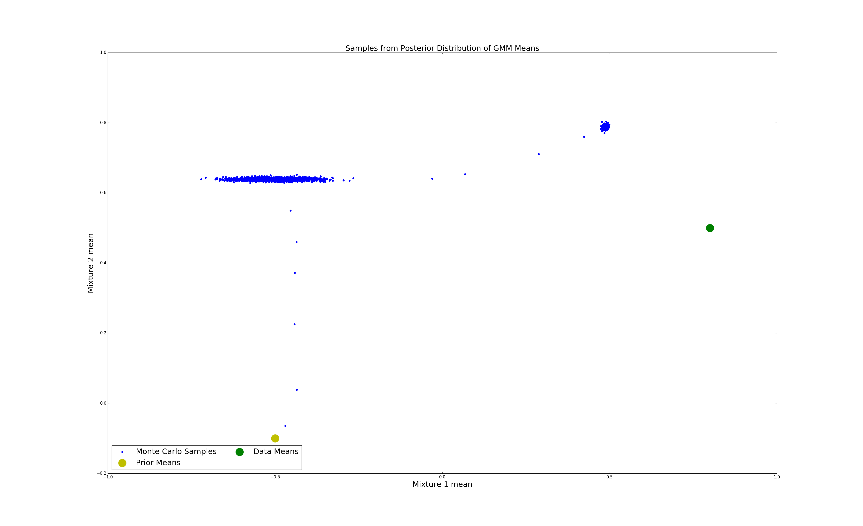
We can plot and visualise the samples of the monte carlo sampler relative to the prior and data means. Note that most of the monte carlo samples are clustered around two areas. These represent the different modes of the distribution.
mc_means = [[s.means[0][0], s.means[1][0]] for s in samples[::10]]
mc_means = np.array(mc_means)

mcmc = plt.scatter(mc_means[:,0], mc_means[:,1], color= 'b')
true = plt.scatter(data_means[0][0], data_means[1][0], color='g', s=500)
prior = plt.scatter(prior_means[0][0], prior_means[1][0], color= 'y', s=500)
plt.title('Samples from Posterior Distribution of GMM Means', fontsize=22)
plt.xlabel('Mixture 1 mean', fontsize=22)
plt.ylabel('Mixture 2 mean', fontsize=22)

plt.legend((mcmc, prior, true),
           ('Monte Carlo Samples', 'Prior Means', 'Data Means'),
           scatterpoints=1,
           loc='lower left',
           ncol=2,
           fontsize=22)

plt.show()